Using the continuum model for the lipid
The LipdBase class
The class rocklinc.lipid.LipdBase handles the generation of the dx
files for the APBS calculations and the reading of the result into
numpy.array.
To customise the lipid model, the user could redefine
rocklinc.lipid.diel_model() to the desirable dielectric constant
profile and rocklinc.lipid.gaussian_mixture() to the desirable
charge density profile.
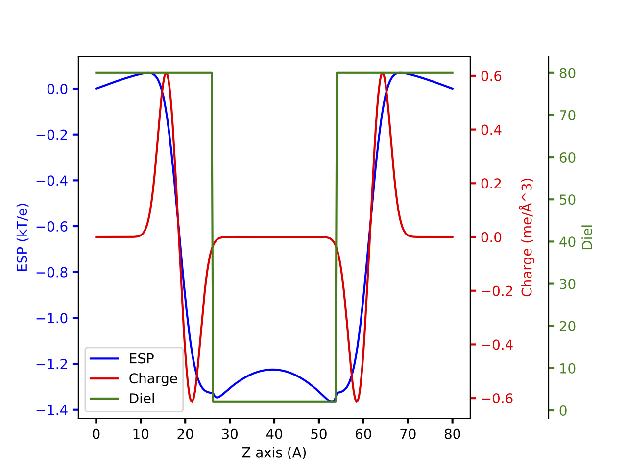
The binary step lipid model
The binary step lipid model is a simple continuum model that is use to describe lipid. The charge is modelled with two Gaussians with opposite magnitude and the dielectric constant is modelled as two region with different dielectric constants.
- rocklinc.lipid.StepLipid.diel_model(x, thickness, diel_low, diel_high)
The dielectric constant with respect to the distance to the end of the lipid.
- Parameters
x (float or array) – The distance to the end of the lipid tail.
thickness (float) – The thickness of the lipid acryl chain, which is the distance from the end of the acryl chain and the begining of the acryl chain.
diel_low (float) – The dielectric constant of the region of the lipid acryl chain.
diel_high (float) – The dielectric constant of the region of the lipid head group and solvent.
- Returns
diel – The one-dimensional array of the dielectric constant.
- Return type
array
- rocklinc.lipid.StepLipid.gaussian_mixture(x, magnitude, neg_loc, neg_width, pos_loc, pos_width)
Charge density with respect to the distance to the end of the lipid.
This functional form is the sum of two Gaussians with opposite magnitude.
- Parameters
x (float or array) – The distance to the end of the lipid tail.
magnitude (float) – The absolute magnitude of both Gaussians (e/Å^3).
neg_loc (float) – The position of the Gaussians with negative magnitude (Å).
neg_width (float) – The spread of the Gaussians with negative magnitude (Å).
pos_loc (float) – The position of the Gaussians with positive magnitude (Å).
pos_width (float) – The spread of the Gaussians with positive magnitude (Å).
- Returns
charge – The one-dimensional array of the charge density.
- Return type
array
The model could be used
import numpy as np
import matplotlib.pyplot as plt
from rocklinc.lipid import StepLipid, plot_dx

lipid = StepLipid([80, 80, 80], [257, 257, 257])
lipid.write_dx_input([6.22602388e-04, 18.5969598, 1.98288109,
                                 24.1998191, 1.91347013],
                      [13.80515, 2, 80])

lipid.write_apbs_input()
lipid.run_APBS()
charge, diel, esp = lipid.read_APBS()
fig = plot_dx(np.linspace(0, lipid.dim[-1].magnitude, lipid.grid[-1]), charge, diel, esp)
plt.show()
Will give a plot looks like this
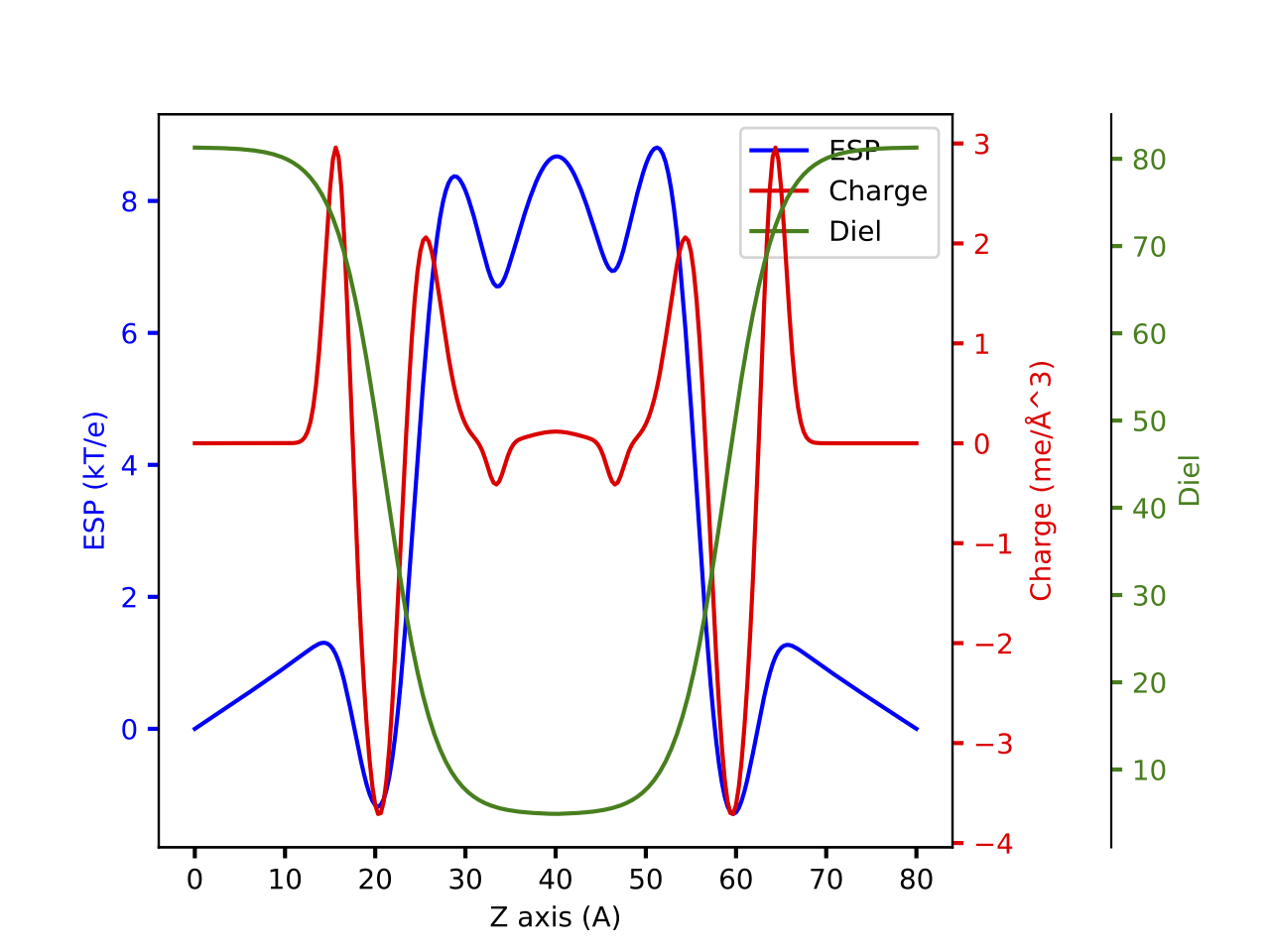
The new lipid model
The new lipid model is a new continuum model that is use to describe lipid. The charge is modelled with five Gaussians to reproduce the complete electrostatic potential profile generated with explicit lipid. The dielectric constant is modelled with logistic function to reproduce the smooth switching from low to high dielectric constant region.
- rocklinc.lipid.CurveLipid.diel_model(x, k1, b1, k2, b2)
The dielectric constant with respect to the distance to the end of the lipid.
- Parameters
x (float or array) – The distance to the end of the lipid tail.
k1 (float) – The slope of the switching from the low to the high dielectric constant region. (1/Å)
b1 (float) – The length of the acryl chain. (Å)
k2 (float) – The dielectric constant of the solvent minus the dielectric constant of the acryl chain of the lipid.
b2 (float) – The dielectric constant of the acryl chain of the lipid.
- Returns
diel – The one-dimensional array of the dielectric constant.
- Return type
array
- rocklinc.lipid.CurveLipid.gaussian_mixture(x, cho_loc, cho_std, cho_mag, po4_loc, po4_std, po4_mag, GL_loc, GL_std, GL_mag, neg_loc, neg_std, neg_mag, pos_std, pos_mag)
Charge density with respect to the distance to the end of the lipid.
This functional form is the sum of two Gaussians with opposite magnitude.
- Parameters
x (float or array) – The distance to the end of the lipid tail.
cho_loc (float) – The position of the Gaussians of the choline group (Å).
cho_std (float) – The spread of the Gaussians of the choline group (Å).
cho_mag (float) – The absolute magnitude of choline group (e/Å^3).
po4_loc (float) – The position of the Gaussians of the phosphate group (Å).
po4_std (float) – The spread of the Gaussians of the phosphate group (Å).
po4_mag (float) – The absolute magnitude of phosphate group (e/Å^3).
GL_loc (float) – The position of the Gaussians of the phosphate group (Å).
GL_std (float) – The spread of the Gaussians of the phosphate group (Å).
GL_mag (float) – The absolute magnitude of phosphate group (e/Å^3).
neg_loc (float) – The position of the Gaussians of the negative dipole of acryl chain (Å).
neg_std (float) – The spread of the Gaussians of negative dipole of acryl chain (Å).
neg_mag (float) – The absolute magnitude of negative dipole of acryl chain (e/Å^3).
pos_std (float) – The spread of the Gaussians with positive dipole of acryl chain (Å).
pos_mag (float) – The absolute magnitude of positive dipole of acryl chain (e/Å^3).
- Returns
charge – The one-dimensional array of the charge density.
- Return type
array
The model could be used
import numpy as np
import matplotlib.pyplot as plt
from rocklinc.lipid import CurveLipid, plot_dx

lipid = CurveLipid([80, 80, 80], [257, 257, 257])
lipid.write_dx_input([24.1998191, 1.28409182, 3.29937546e-03,
                      18.5969598, 2.41286946, 5.70594706e-03,
                      16.0770291, 2.47034776, 4.17737240e-03,
                      6.59972225, 0.90515386, 4.25321040e-04,
                      2.95472778, 1.17224618e-04],
                      [0.36626031, 18.87278382, 76.49060424, 4.83151723])

lipid.write_apbs_input()
lipid.run_APBS()
charge, diel, esp = lipid.read_APBS()
fig = plot_dx(np.linspace(0, lipid.dim[-1].magnitude, lipid.grid[-1]), charge, diel, esp)
plt.show()
Will give a plot looks like this
API Reference
- class rocklinc.lipid.LipdBase(dim, grid)[source]
setup the grids for the APBS calculations.
- Parameters
dim (list) – The unitcell dimensions of the system in Å
[lx, ly, lz]. The pq.Quantity array could also be used.grid (list) – The number of grids in the x, y, z axis
[257, 257, 257].
- static diel_model(x, **kwargs)[source]
The dielectric constant with respect to the distance to the end of the lipid.
- Parameters
x (float or array) – The distance to the end of the lipid tail.
**kwargs (dict) – Additional keyword arguments.
- Returns
diel – The one-dimensional array of the dielectric constant.
- Return type
array
- static gaussian_mixture(x, **kwargs)[source]
Charge density with respect to the distance to the end of the lipid.
- Parameters
x (float or array) – The distance to the end of the lipid tail.
**kwargs (dict) – Additional keyword arguments.
- Returns
charge – The one-dimensional array of the charge density.
- Return type
array
- generate_charge(z_list, param_charge)[source]
Generate the charge density from the coordinates.
- Parameters
z_list (array) – The one-dimensional coordinate array.
**kwargs (dict) – Additional keyword arguments.
- Returns
charge – The one-dimensional array of the charge density.
- Return type
array
- generate_diel(z_list, param_diel)[source]
Generate the dielectric constant from the coordinates.
- Parameters
z_list (array) – The one-dimensional coordinate array.
**kwargs (dict) – Additional keyword arguments.
- Returns
diel – The one-dimensional array of the dielectric constant.
- Return type
array
- read_APBS()[source]
Read the APBS output.
- Returns
charge (array) – The three-dimensional array of the charge density.
diel (array) – The three-dimensional array of the dielectric constant in the x direction.
lipid (array) – The three-dimensional array of the ESP.
- read_central_ESP()[source]
Read the one-dimensional ESP along the Z-axis at the center of the x-y plane.
- Returns
out_ESP – The one-dimensional ESP.
- Return type
array
- run_APBS(apbs_exe='/opt/local/bin/apbs', apbs_in='lipid.in')[source]
Running the APBS calculations, which is the same as
apbs lipid.in
- Parameters
apbs_exe (str, optional) – The path to the APBS program. (
/opt/local/bin/apbs)apbs_in (str, optional) – The input file to the APBS program. (
lipid.in)
- write_apbs_input()[source]
Generate the APBS input file
lipid.inand the reference qpr fileref.pqr.The APBS calculation will use the
dielx.dx,diely.dxanddielz.dxfor dielectric constant andcharge.dxfor the charge density. Theref.pqris a place holder and is not used in the calculation.
- write_dx_input(param_charge, param_diel)[source]
Generate the dielectric constant and charge grid for APBS calculations.
generate_chargeandgenerate_dielare used to generate the profile of the charge and dielectric constant on the one-dimensional z-axis which is then broadcast to cover the whole 3D space. The generated files are named asdielx.dx,diely.dx,dielz.dxandcharge.dx.- Parameters
**kwargs (dict) –
generate_chargeuses the arguments from kwargs[‘charge’] andgenerate_dieluses the arguments from kwargs[‘diel’].